ELATE Object Usage
In the previous page there were quick snippits of code to start getting results quickly. Here, we will do a step by step example to explain all the features the ELATE implementation has to offer. The original website for ELATE can be found here, <http://progs.coudert.name/elate>.
1.1 Initialization of the ELATE object
To start off, we need to import the necessary packages that we will use in the example. We will use the ELATE object class from mechelastic.core, which can be thought of as a container for all the calculations for the ELATE code. We will also use pyvista to demonstrate how one can easily access the 3D meshes directly to customize as they please. Finally, we will use a direct elastic tensor for this example. This elastic tensor was calculated with VASP on bulk silicon and can be found in the examples folder. For direct elastic tensor input, the proper format is a list of lists containing the elastic constants. We also have the density of this structure because this will allow us to display thermal properties. The density must be in units kg/m^3
Importing ELATE object:
>>> from mechelastic.core import ELATE
>>> import pyvista as pv
>>> elastic_tensor =[
>>> [153.1305, 56.7932  , 56.7932  ,  0.0000  , 0.0000  , -0.0000   ],
>>> [56.7932 , 153.1305 , 56.7932  , -0.0000  , -0.0000 , -0.0000   ],
>>> [56.7932 , 56.7932  , 153.1305 , -0.0000  , 0.0000  , 0.0000   ],
>>> [0.0000  , -0.0000  , -0.0000  , 74.7184  , -0.0000 , 0.0000   ],
>>> [0.0000  , -0.0000  , 0.0000   , -0.0000  , 74.7184 , 0.0000   ],
>>> [-0.0000 , -0.0000  , 0.0000   , 0.0000   , 0.0000  , 74.7184 ],
>>> ]
>>> density = 2281.05840 # in kg/m^3
We may initialize the ELATE object with the elastic tensor and the density. The density is not required and may be set to None if one does not have density information.
Initialization of ELATE object:
>>> elate = ELATE(s = elastic_tensor, density = density)
Note
If one wants to use a DFT code output for this example. They need to use the appropriate parser from mechelastic.parsers to get the density and the elastic tensor
1.2 Interacting with the ELATE object
From this object we can access the entire ELATE code by calling the class methods and attributes. We will first start by calling the print_properties() method to view a summary of the ELATE analysis to see which quantities we can access.
1.2.1 Print Summary
Usage :
>>> elate.print_properties()
Output
        Average properties


                 Voigt     Reuss    Hill
-------------------------------------------------------
Bulk modulus       (GPa)      88.906    88.906    88.906
Shear modulus      (GPa)      64.097    61.220    62.659
Young's modulus    (GPa)      155.034   149.374   152.216
Poisson's ratio               0.209     0.220     0.215
Pugh's Ratio                  1.387     1.452     1.419
Compression Speed  (m/s)      8743.125  8646.400  8694.897
Shear Speed        (m/s)      5300.929  5180.575  5241.098
Ratio Vc/Vs                   2.720     2.786     2.752
Debye Speed        (m/s)      4688.006  4598.120  4643.367
-------------------------------------------------------


Eigenvalues of compliance matrix


   lamda_1  lamda_2  lamda_3  lamda_4  lamda_5  lamda_6
---------------------------------------------------------------
   74.717    74.717    74.717    96.336    96.336   266.718
--------------------------------------------------------------


Variations of the elastic moduli


                                  Min       Max   ||   Anisotropy
----------------------------------------------------------------------------------------
Young's Modulus     (GPa)        122.399   175.100 ||    1.431
         Min Axis:    (0.0, 0.0, 1.0)
         Max Axis:    (0.577, 0.577, -0.577)
----------------------------------------------------------------------------------------
Linear Compression   (TPa^-1)      3.749     3.749 ||    1.000
         Min Axis:    (0.958, 0.126, 0.259)
         Max Axis:    (0.5, 0.5, 0.707)
----------------------------------------------------------------------------------------
Bulk Modulus   (GPa,Experimental)             38.418   223.191 ||    5.810
         Min Axis:    (0.707, -0.0, 0.707)
         Max Axis:    (0.707, -0.001, 0.707)
         Second Min Axis:    (0.707, -0.001, -0.707)
         Second Max Axis:    (0.707, -0.001, -0.707)
----------------------------------------------------------------------------------------
Shear Modulus   (GPa)             48.168    74.717 ||    1.551
         Min Axis:    (0.707, -0.0, 0.707)
         Max Axis:    (0.0, 0.0, 1.0)
         Second Min Axis:    (0.707, -0.001, -0.707)
         Second Max Axis:    (0.707, -0.001, -0.707)
----------------------------------------------------------------------------------------
Poisson's Ratio                     0.058     0.349 ||    6.037
         Min Axis:    (0.707, -0.0, 0.707)
         Max Axis:    (0.707, -0.001, 0.707)
         Second Min Axis:    (0.707, -0.001, -0.707)
         Second Max Axis:    (0.0, 1.0, 0.0)
----------------------------------------------------------------------------------------
Pugh's Ratio                    1.190     1.846 ||    1.551
         Min Axis:    (0.0, 0.0, 1.0)
         Max Axis:    (0.707, -0.0, 0.707)
         Second Min Axis:    (0.174, 0.985, -0.0)
         Second Max Axis:    (0.174, 0.985, -0.0)
----------------------------------------------------------------------------------------
Compression Speed                  8193.358  9091.185 ||    1.110
         Min Axis:    (0.707, -0.0, 0.707)
         Max Axis:    (0.0, 0.0, 1.0)
         Second Min Axis:    (0.707, -0.001, -0.707)
         Second Max Axis:    (1.0, 0.0, -0.0)
----------------------------------------------------------------------------------------
Shear Speed                  4595.271  5723.234 ||    1.245
         Min Axis:    (0.707, -0.0, 0.707)
         Max Axis:    (0.0, 0.0, 1.0)
         Second Min Axis:    (0.707, -0.001, -0.707)
         Second Max Axis:    (1.0, 0.0, -0.0)
----------------------------------------------------------------------------------------
Ratio Compression Shear Speed                     2.523     3.179 ||    1.260
         Min Axis:    (0.0, 0.0, 1.0)
         Max Axis:    (0.707, -0.0, 0.707)
         Second Min Axis:    (0.174, 0.985, -0.0)
         Second Max Axis:    (0.707, -0.001, -0.707)
----------------------------------------------------------------------------------------
Debye Speed                  4154.917  5000.827 ||    1.204
         Min Axis:    (0.707, -0.0, 0.707)
         Max Axis:    (0.0, 0.0, 1.0)
         Second Min Axis:    (0.707, -0.001, -0.707)
         Second Max Axis:    (0.174, 0.985, -0.0)
1.2.2 Accessing quantities
There are two ways to access any given quantity in the print summary, either call the wanted quantity as an attribute or through the to_dict() method.
Attribute Usage:
>>> voigt_bulk = elate.voigtK
>>> reuss_bulk = elate.reussK
>>> hill_bulk  = elate.hillK
>>> anisotropy_poisson = elate.anis_Poisson
>>> print(f"Voigt Bulk modulus : {voigt_bulk} GPa")
>>> print(f"Reuss Bulk modulus : {reuss_bulk} GPa")
>>> print(f"Hill Bulk modulus : {hill_bulk} GPa")
>>> print(f"Anisotropy in Poisson's Ratio : {anisotropy_poisson}")
Output:
Voigt Bulk modulus : 88.90563333333334 GPa
Reuss Bulk modulus : 88.90563333333334 GPa
Hill Bulk modulus : 88.90563333333334 GPa
Anisotropy in Poisson`s Ratio : 6.037439233255422
Above was just an example of the different attributes available, but to see what other attributes are available use dir(elate)
to_dict() Usage:
>>> elate_dict = elate.to_dict()
>>> for key in elate_dict.keys():
>>>     print(key + ':', elate_dict[key])
Output:
bulk_modulus_voigt: 88.90563333333334
bulk_modulus_reuss: 88.90563333333336
bulk_modulus_hill: 88.90563333333336
bulk_max: 223.18983956287462
bulk_min: 38.41779228916066
bulk_min_axis: (0.7070890777249003, -3.2660969780252564e-05, -0.7071244834506942)
bulk_max_axis: (-0.7071011747765165, -2.7858572302977706e-05, 0.7071123870033463)
bulk_min_axis_2: (-0.7071244601718366, 0.00022805942991048573, -0.7070890649809153)
bulk_max_axis_2: (3.792727173859518e-05, -0.9999999992796791, -1.4709880630005777e-06)
bulk_anisotropy: 5.809543606331753
youngs_modulus_voigt: 155.03649359718446
youngs_modulus_reuss: 149.37560549227936
youngs_modulus_hill: 152.2184138933355
youngs_max: 175.1019299786047
youngs_min: 122.40059607547886
youngs_min_axis: (0.0, 0.0, 1.0)
youngs_max_axis: (-0.577361569343, 0.5773687973343659, 0.5773204397130386)
youngs_anisotropy: 1.4305643566525388
linearCompression_max: 3.7492937267942166
linearCompression_min: 3.749293726794212
linearCompression_min_axis: (-0.49500029477676866, 0.8573656603149349, -0.1410632222928697)
linearCompression_max_axis: (0.5000000000000001, 0.5000000000000001, 0.7071067811865476)
linearCompression_anisotropy: 1.000000000000001
shear_modulus_voigt: 64.09850000000002
shear_modulus_reuss: 61.22084076167894
shear_modulus_hill: 62.65967038083948
shear_max: 74.71840000000003
shear_min: 48.16865095136881
shear_min_axis: (0.7070890649809153, 0.0001381629613373221, -0.7071244834506942)
shear_max_axis: (0.0, 0.0, 1.0)
shear_min_axis_2: (-0.7071244601718367, -0.00018436062115480075, -0.7070890777249003)
shear_max_axis_2: (0.17364817766693041, 0.9848077530122079, -0.0)
shear_anisotropy: 1.5511831559375808
poisson_modulus_voigt: 0.20936132356595238
poisson_modulus_reuss: 0.21997348969585478
poisson_modulus_hill: 0.21464422784357595
poisson_max: 0.3494163383468135
poisson_min: 0.057874924259636105
poisson_min_axis: (0.7070890777249003, -3.2660969780252564e-05, -0.7071244834506942)
poisson_max_axis: (-0.7070718209701229, 1.3417388323657962e-05, 0.7071417395472906)
poisson_min_axis_2: (-0.7071244601718366, 0.00022805942991048573, -0.7070890649809153)
poisson_max_axis_2: (-1.3289480480657114e-05, -0.9999999998955298, 5.685947999088838e-06)
poisson_anisotropy: 6.03743923325543
pugh_ratio_voigt: 1.387015816802785
pugh_ratio_reuss: 1.4522118975697513
pugh_ratio_hill: 1.4188653210745192
pugh_ratio_max: 1.8457156589893435
pugh_ratio_min: 1.1898760323204636
pugh_ratio_min_axis: (0.0, 0.0, 1.0)
pugh_ratio_max_axis: (0.7070890649809153, 0.0001381629613373221, -0.7071244834506942)
pugh_ratio_min_axis_2: (0.17364817766693041, 0.9848077530122079, -0.0)
pugh_ratio_max_axis_2: (-0.7071244601718367, -0.00018436062115480075, -0.7070890777249003)
pugh_ratio_anisotropy: 1.5511831559375808
compressionSpeed_voigt: 8743.152534460714
compressionSpeed_reuss: 8646.424429285951
compressionSpeed_hill: 8694.9229913841
compressionSpeed_max: 9091.221174861093
compressionSpeed_min: 8193.371731108246
compressionSpeed_min_axis: (0.7070810029832681, -0.00026317043674738697, 0.7071325094785961)
compressionSpeed_max_axis: (0.0, 0.0, 1.0)
compressionSpeed_anisotropy: 1.109582412859889
shearSpeed_voigt: 5300.974695538509
shearSpeed_reuss: 5180.616478819788
shearSpeed_hill: 5241.141088701903
shearSpeed_max: 5723.28772470741
shearSpeed_min: 4595.301802302283
shearSpeed_min_axis: (0.7070890649809153, 0.0001381629613373221, -0.7071244834506942)
shearSpeed_max_axis: (0.0, 0.0, 1.0)
shearSpeed_anisotropy: 1.245465036015697
ratioCompressionShearSpeed_voigt: 2.720349150136119
ratioCompressionShearSpeed_reuss: 2.785545230903085
ratioCompressionShearSpeed_hill: 2.7521986544078523
ratioCompressionShearSpeed_max: 3.1790489923226763
ratioCompressionShearSpeed_min: 2.523209365653796
ratioCompressionShearSpeed_min_axis: (0.0, 0.0, 1.0)
ratioCompressionShearSpeed_max_axis: (0.7070890649809153, 0.0001381629613373221, -0.7071244834506942)
ratioCompressionShearSpeed_anisotropy: 1.2599227934059858
debyeSpeed_voigt: 4688.038385364817
debyeSpeed_reuss: 4598.1495576239095
debyeSpeed_hill: 4643.39765995238
debyeSpeed_max: 5000.864516324726
debyeSpeed_min: 4154.939222859331
debyeSpeed_min_axis: (0.7070890649809153, 0.0001381629613373221, -0.7071244834506942)
debyeSpeed_max_axis: (0.0, 0.0, 1.0)
debyeSpeed_anisotropy: 1.2035951064726405
As you can see, one can easily access whatever quantity they need through this method.
1.2.3 Plotting Methods
In ELATE’s website they provide the 2d cross sectional plots and the 3d visualizations of the Young’s Modulus, Linear Compression, Shear Modulus, and Poisson’s Ratio. This funcationality is still availible in mechelastic, through the plot_2D() and thye plot_3D() methods. The input of this method is the specific elastic property you want to plot and wether you want show the plot. MechElastic now has a 3d slicing widget which can make 2d cross sectional cuts of the 3D surface through the plot_3D_slice().
The available properties to plot : “BULK”, POISSON” , “SHEAR”, “YOUNG” , “LC” ,”PUGH_RATIO”. If the density is provided, then one can also plot : “COMPRESSION_SPEED” , “SHEAR_SPEED” , “RATIO_COMPRESSIONAL_SHEAR” , “DEBYE_SPEED”
Note
If there are any kinks in the plots, this is due to even or odd number of points used. By using the parameter npoints one can change the number of points used.
plot_2D() Usage:
>>> fig = elate.plot_2D(elastic_calc = "POISSON", show = True )
Output:

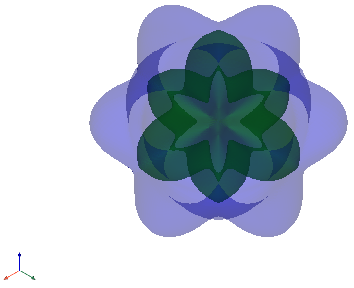
plot_3D() Usage
>>> meshes = elate.plot_3D(elastic_calc = "POISSON", show = True)
Output:
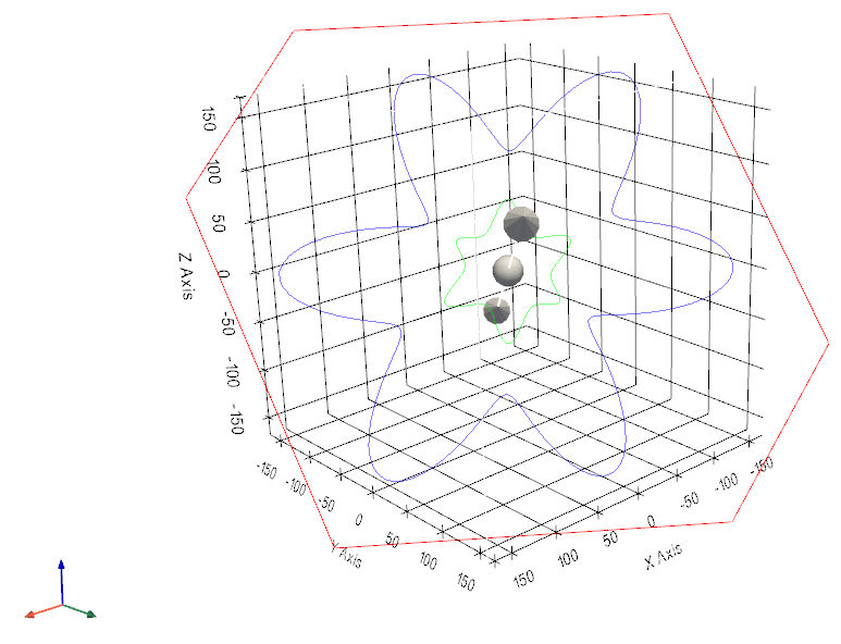
plot_3D_slice() Usage
>>> meshes = elate.plot_3D_slice(elastic_calc = "POISSON", normal = (1,0,0), show = True)
Output: