Band structure¶

PyProcar goes beyond the conventional plain band structure to plot the projected bands that carry even more information. The projected bands are color coded in an informative manner to portray fine details.

1. Plain band structure¶

This is the most basic type of band structure. No projection information is contained here. In order to use the plain mode one sets mode='plain'. elimit sets the energy window limits. outcar specifies the OUTCAR file. For Abinit calculations, abinit_output is used instead. color lets the user use any color available in the matplotlib package. If an output file is not present one can set fermi manually. One may save the plot using the savefig tag, for example, savefig='figure.png' with a desired image file format. This applies to all other band structure plotting functions in PyProcar as well. For Elk, setting file=’PROCAR’ and outcar=’OUTCAR’ is not necessary. As long as the path to elk.in is defined or PyProcar is executed in the directory of calculation, PyProcar will work of the files needed for the bandsplot.

Usage:

pyprocar.bandsplot('PROCAR',outcar='OUTCAR',elimit=[-2,2],mode='plain',color='blue',code='vasp')

PyProcar is capable of labeling the \(k\)-path names automatically, however, the user can manually input them as desired.

If a KPOINTS file is present automatic labeling can be enabled as follows:

pyprocar.bandsplot('PROCAR',outcar='OUTCAR',elimit=[-2,2],mode='plain',color='blue',kpointsfile='KPOINTS')

For VASP, the KPOINTS file should be similar to the following:

UCB (simple cubic) G-X-M-G-R-X M-R
 ! 40 grids
Line-mode
reciprocal
0000   0.0000   0.0000   ! \Gamma
0000   0.5000   0.0000   ! X

0000   0.5000   0.0000   ! X
5000   0.5000   0.0000   ! M

5000   0.5000   0.0000   ! M
0000   0.0000   0.0000   ! \Gamma

0000   0.0000   0.0000   ! \Gamma
5000   0.5000   0.5000   ! R

5000   0.5000   0.5000   ! R
0000   0.5000   0.0000   ! X

For Elk, to retrieve the KPOINTS automatically, one should define the \(k\)-path block in the elk.in file such as:

! These are the vertices to be joined for the band structure plot
plot1d
50
0      0.0      0.0 : \Gamma
5      0.0      0.0 : X
5      0.5      0.0 : M
0      0.0      0.0 : \Gamma
5      0.5      0.5 : R
5      0.0      0.0 : X

In Quantum Espresso, it should be define in a similar way. Check the examples directory for more information.

One may manually label the \(k\)-path as well. knames and kticks corresponds to the labels and the number of grid points between the high symmetry points in the \(k\)-path used for the band structure calculation. Usage:

pyprocar.bandsplot('PROCAR',outcar='OUTCAR',elimit=[-2,2],mode='plain',color='blue',kticks=[0,39,79,119,159],knames=['G','X','M','G','R'],code='vasp')

This is valid for the rest of the band plotting modes as well.

2. Spin projection¶

For collinear spin polarized and non-collinear spin calculations of DFT codes, PyProcar is able to plot the bands considering spin density (magnitude), spin magnetization and spin channels separately.

For non-collinear spin calculations, spin=0 plots the spin density (magnitude) and spin=1,2,3 corresponds to spins oriented in \(S_x\), \(S_y\) and \(S_z\) directions respectively. Setting spin='st' plots the spin texture perpendicular in the plane (\(k_x\), \(k_y\)) to each (\(k_x\),i \(k_y\)) vector. This is useful for Rashba-like states in surfaces. For parametric plots such as spin, atom and orbitals, the user should set mode=`parametric'. cmap refers to the matplotlib color map used for the parametric plotting and can be modified by using the same color maps used in matplotlib. cmap='seismic' is recommended for parametric spin band structure plots. For colinear spin calculations setting spin=0 plots the spin density (magnitude) and spin=1 plots the spin magnetization. Spin channels can also be plot separately (see below).

Usage:

pyprocar.bandsplot('PROCAR',outcar='OUTCAR',elimit=[-5,5],kticks=[0,39,79,119,159],knames=['G','X','M','G','R'],cmap='jet',mode='parametric',spin=1)

If spin-up and spin-down bands are to be plot separately (for colinear calculations), there are two methods one can follow.

The pyprocar.filter() function can be used to create two PROCARs for each spin direction and be plot individually. An example is given below:

pyprocar.filter('PROCAR','PROCAR-up',spin=[0])
pyprocar.filter('PROCAR','PROCAR-down',spin=[1])
pyprocar.bandsplot('PROCAR-up',...)
pyprocar.bandsplot('PROCAR-down',...)

Setting the separate=True parameter in pyprocar.bandsplot() plots spin up bands and spin down bands with spin=0 and spin=1, respectively.

E.g.:

pyprocar.bandsplot('PROCAR',mode='parametric',separate=True,spin=0,...)

These methods can be used for both plain and parametric modes. If a comparison of spin up and spin down bands is required on the same plot, the following syntax can be used.

E.g.:

fig, ax = pyprocar.bandsplot('PROCAR-up',show=False,color='red',mode='plain')
pyprocar.bandsplot('PROCAR-down',color='blue',mode='plain',ax=ax)

Note:

Currently, Elk only supports spin colinear plotting. Non colinear spin plotting will be implemented in the future.

3. Atom projection¶

The projection of atoms onto bands can provide information such as which atoms contribute to the electronic states near the Fermi level. PyProcar counts each row of ions in the PROCAR file, starting from zero. In an example of a five atom SrVO:math:_3, the indexes of atoms for Sr, V and the three O atoms would be 0,1 and 2,3,4 respectively. It is also possible to include more than one type of atom by using an array such as atoms = [0,1,3]. The index 5 would correspond to the total contribution from all the atoms.

Usage:

pyprocar.bandsplot('PROCAR',outcar='OUTCAR',elimit=[-5,5],kticks=[0,39,79,119,159],knames=['G','X','M','G','R'],cmap='jet', mode='parametric',atoms=[1])

NOTE:

The reason for this format which includes the “total” atomic contribution as the last atom index is because the PROCAR file from VASP which PyProcar was originally based on had a “tot” row for each k-point/band block that summed up all the atom contributions. So the parser was meant to incorporate that as well. The other DFT parsers followed suit to be consistent with this format.

4. Orbital projection¶

The projection of atomic orbitals onto bands is also useful to identify the contribution of orbitals to bands. For instance, to identify correlated \(d\) or \(f\) orbitals in a strongly correlated material near the Fermi level. It is possible to include more than one type of orbital projection. The mapping of the index of orbitals to be used in orbitals is as follows (this is the same order from the PROCAR file). Quantum Espresso, VASP and Abinit follows this order.

In Elk, the \(Y_{lm}\) projections of the atomic site resolved DOS are arranged in logical order in the BAND_S*A* files, namely: (l,m) = (0,0), (1,-1), (1,0), (1,1), (2,-2), (2,-1), (2,0), (2,1), (2,2), etc.,

Usage: To project all five \(d\)-orbitals:

pyprocar.bandsplot('PROCAR',outcar='OUTCAR',elimit=[-5,5],kticks=[0,39,79,119,159],knames=['G','X','M','G','R'],cmap='jet',mode='parametric',orbitals=[4,5,6,7,8])

One or many of the above can be combined together to allow the user to probe into more specific queries such as a collinear spin projection of a certain orbital of a certain atom.

Different modes of band structures are useful for obtaining information for different cases. The four modes available within PyProcar are plain, scatter, parametric and atomic. The plain bands contain no projection information. The scatter mode creates a scatter plot of points. The parametric mode interpolates between points to create bands which are also projectable. Finally, the atomic mode is useful to plot energy levels for atoms. To set maximum and minimum projections for color map, one could use vmin and vmax tags.

Export plot as a matplotlib.pyplot object¶

PyProcar allows the plot to be exported as a matplotlib.pyplot object. This allows for further processing of the plot through options available in matplotlib. Usage:

fig, ax = pyprocar.bandsplot('PROCAR', outcar='OUTCAR', mode='plain', show=False)
ax.set_title('Using matplotlib options')
fig.show()

Converting \(k\)-points from reduced to cartesian coordinates¶

PyProcar defaults to plotting using the reduced coordinates of the \(k\)-points. If one wishes to plot using cartesian coordinates, set kdirect=False. However, an OUTCAR must be supplied for this case to retrieve the reciprocal lattice vectors to transform the coordinates from reduced to cartesian. Note that for the case of Elk, the output is automatically retrieved so it is not necessary to provide it for the conversion.

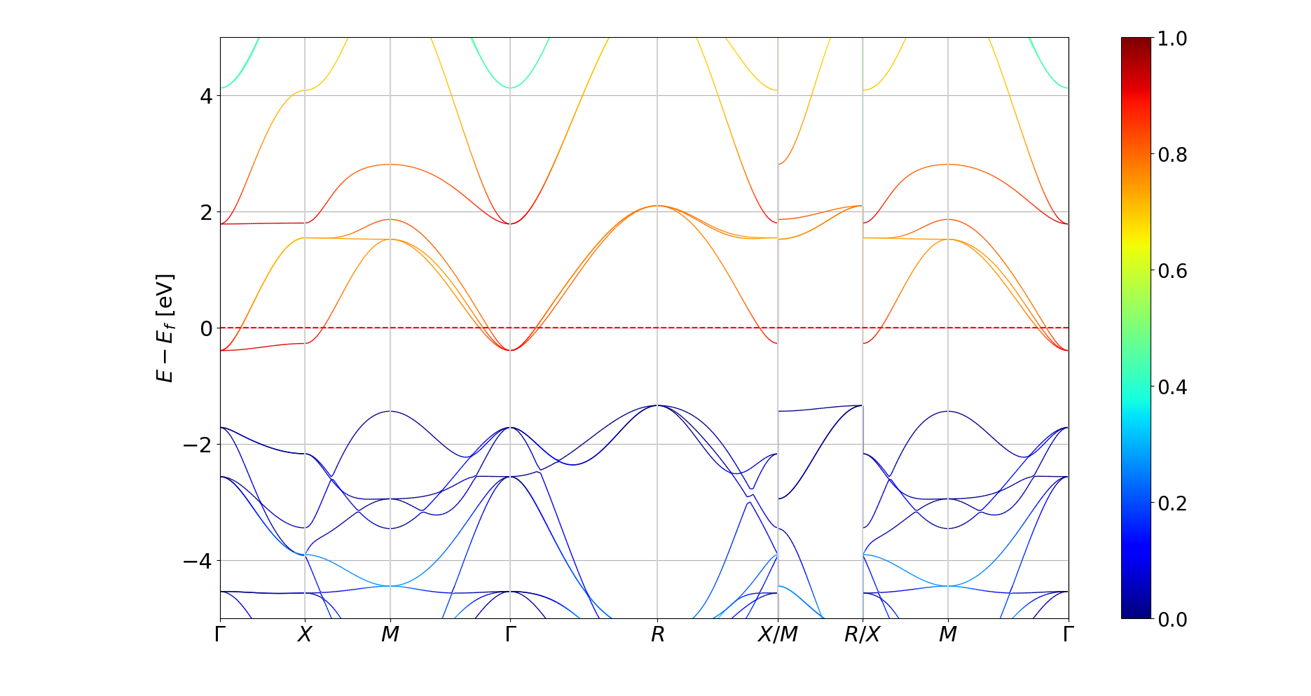
Plotting band structures with a discontinuous \(k\)-path¶

PyProcar allows the plotting of band structures with a discontinuous \(k\)-path. If a KPOINTS file with the \(k\)-path is supplied, PyProcar will automatically find the \(k\)-point indices where the discontinuities occur. If not, one may manually set it with the discontinuities variable. For example, the \(k\)-path G-X-M-G-R-X M-R X-M-G with 40 grid points should be set as:

knames = ['$\\Gamma$', '$X$', '$M$', '$\\Gamma$', '$R$', '$X/M$', '$R/X$', '$M$', '$\\Gamma$']
kticks = [0, 39, 79, 119, 159, 199, 239, 279, 319]
discontinuities = [199, 239]

pyprocar.scriptBandsplot.bandsplot(procar='PROCAR', abinit_output='abinit.out', dirname=None, poscar=None, outcar=None, kpoints=None, elkin='elk.in', code='vasp', mode='plain', spins=None, atoms=None, orbitals=None, items=None, fermi=None, interpolation_factor=1, interpolation_type='cubic', projection_mask=None, vmax=None, vmin=None, kticks=None, knames=None, kdirect=True, elimit=None, ax=None, show=True, savefig=None, old=False, **kwargs)[source]¶

Parameters

procar (TYPE, optional) – DESCRIPTION. The default is “PROCAR”.
abinit_output (TYPE, optional) – DESCRIPTION. The default is “abinit.out”.
outcar (TYPE, optional) –

DESCRIPTION. The default is “OUTCAR”.
kpoints : TYPE, optional

DESCRIPTION. The default is “KPOINTS”.
elkin (TYPE, optional) – DESCRIPTION. The default is “elk.in”.
mode (TYPE, optional) – DESCRIPTION. The default is “plain”.
spin_mode (TYPE, optional) – plain, magnetization, density, “spin_up”, “spin_down”, “both”, “sx”, “sy”, “sz”, “spin_texture” DESCRIPTION. The default is “plain”.
spins (TYPE, optional) – DESCRIPTION.
atoms (TYPE, optional) – DESCRIPTION. The default is None.
orbitals (TYPE, optional) – DESCRIPTION. The default is None.
fermi (TYPE, optional) – DESCRIPTION. The default is None.
mask (TYPE, optional) – DESCRIPTION. The default is None.
colors (TYPE, optional) – DESCRIPTION.
cmap (TYPE, optional) – DESCRIPTION. The default is “jet”.
marker (TYPE, optional) – DESCRIPTION. The default is “o”.
markersize (TYPE, optional) – DESCRIPTION. The default is 0.02.
linewidth (TYPE, optional) – DESCRIPTION. The default is 1.
vmax (TYPE, optional) – DESCRIPTION. The default is None.
vmin (TYPE, optional) – DESCRIPTION. The default is None.
grid (TYPE, optional) – DESCRIPTION. The default is False.
kticks (TYPE, optional) – DESCRIPTION. The default is None.
knames (TYPE, optional) – DESCRIPTION. The default is None.
elimit (TYPE, optional) – DESCRIPTION. The default is None.
ax (TYPE, optional) – DESCRIPTION. The default is None.
show (TYPE, optional) – DESCRIPTION. The default is True.
savefig (TYPE, optional) – DESCRIPTION. The default is None.
plot_color_bar (TYPE, optional) – DESCRIPTION. The default is True.
title (TYPE, optional) – DESCRIPTION. The default is None.
kdirect (TYPE, optional) – DESCRIPTION. The default is True.
code (TYPE, optional) – DESCRIPTION. The default is “vasp”.
lobstercode (TYPE, optional) – DESCRIPTION. The default is “qe”.
verbose (TYPE, optional) – DESCRIPTION. The default is True.

Returns

Return type

None.