Autobands plotting

One of the most powerful capabilities of PyProcar is allowing to correlate real space with electronic structure, for instance finding surface states or defect levels. Traditionally this task is done by the user, providing a list of atoms representing the surface or the defect (parameter atom in bandsplot). Also the user needs to choose a relevant energy window for the plot and setting the boundaries of the color scale to highlight the relevant states. That process is both tedious and error prone: for instance the user need to find the special atoms (e.g. defect, surface, etc.) and take care of whether the indexes are 0- or 1-based.

Specifically, the function aims to: - Determine an optimal energy window for the plot, which includes bulk-like bands both above and below the fundamental band gap for insulators, as well as any localized states within that gap. - Identify important real-space features such as defects, surfaces, and van der Waals layers. - Locate localized electronic states within the selected energy window. - Calculate suitable values for the color map to emphasize these localized states.

All these tasks are executed without requiring user intervention. The identification of real-space features is carried out using PyPoscar. Localized states are identified through the Inverse Participation Ratio (IPR). The function correlates the geometry and electronic structure by evaluating the participation of relevant atoms in the IPR calculations.

This automated identification of key features is most effective when the atoms of interest are statistically distinct from the rest of the system, both in real space and electronic structure. In scenarios where such distinctions are not readily apparent, the function will default to generating a standard band structure plot. It’s important to note that while our current implementation is robust, there may be some geometrical features it does not yet capture. However, we anticipate that the function will continue to improve based on user feedback.

Preparation

Before diving into plotting, we need to download the example files. Use the following code to do this. Once downloaded, specify the data_dir to point to the location of the downloaded data.

Downloading example

 import pyprocar

 bi2se3_data_dir = pyprocar.download_example(
                             save_dir='',
                             material='auto',
                             code='vasp',
                             spin_calc_type='non-spin-polarized',
                             calc_type='bands'
                            )

Setting up the environment

First, we will import the necessary libraries and set up our data directory path.

import os
import pyprocar

# Define the directory containing the example data
data_dir = f"{pyprocar.utils.ROOT}{os.sep}data{os.sep}examples{os.sep}auto"

Autobands Example

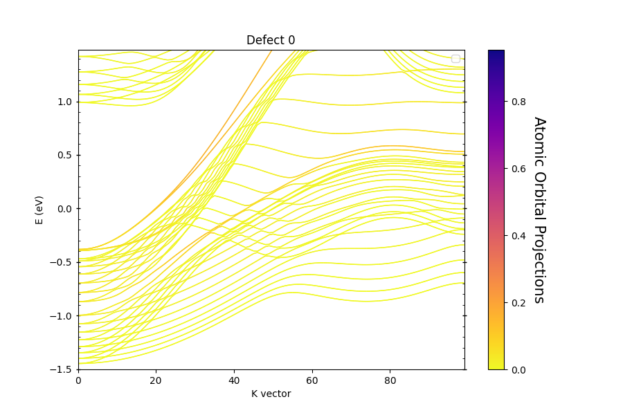
As an example of this functionality, we calculate a slab of a topologically non-trivial phase of Bi. It features surface states with Dirac cones at high-symmetry points. The code used to plot the band structure is below. The title of the figure is Defect 0, which corresponds to the upper surface of the slab, the other surface generates a second figure, with title Defect 1. When running the code above, a file report.txt is generated with info about the atoms comprising each defect, and the associated localized states.

pyprocar.autobandsplot(code='vasp', dirname=data_dir)

• 
• 

2 orbitals. (Some of) They are unknow (if you did 'filter' them it is OK).
[[0, 0.953], [0, 0.956]]
[]

            ----------------------------------------------------------------------------------------------------------
            There are additional plot options that are defined in the configuration file.
            You can change these configurations by passing the keyword argument to the function.
            To print a list of all plot options set `print_plot_opts=True`

            Here is a list modes : plain , parametric , scatter , atomic , overlay , overlay_species , overlay_orbitals , ipr
            ----------------------------------------------------------------------------------------------------------

2 orbitals. (Some of) They are unknow (if you did 'filter' them it is OK).

            WARNING : `fermi` is not set! Set `fermi={value}`. The plot did not shift the bands by the Fermi energy.
            ----------------------------------------------------------------------------------------------------------


            ----------------------------------------------------------------------------------------------------------
            There are additional plot options that are defined in the configuration file.
            You can change these configurations by passing the keyword argument to the function.
            To print a list of all plot options set `print_plot_opts=True`

            Here is a list modes : plain , parametric , scatter , atomic , overlay , overlay_species , overlay_orbitals , ipr
            ----------------------------------------------------------------------------------------------------------

2 orbitals. (Some of) They are unknow (if you did 'filter' them it is OK).

            WARNING : `fermi` is not set! Set `fermi={value}`. The plot did not shift the bands by the Fermi energy.
            ----------------------------------------------------------------------------------------------------------