Plotting Inverse participation ratio

Often it is needed to search for localized modes within the band structure, typical examples are surface/interface states and defect levels. The usual procedure for detecting them is looking for bands with a large projection around the atoms at the surface or defect. This procedure is both cumbersome for the user and error-prone. For instance, the lowest unoccupied levels of the neutral \(C_N\) defect in h-BN has practically no projection on the defect atom and its nearest neighbors. This delayed its identification as a single-photon emitter.[jara2021,auburger2021] A much simpler way to detect these localized levels is by means of the Inverse Participation Ratio, defined as

\[IPR_{nk} = \frac{\sum_{a} |c_{nki}|^4}{\left(\sum_a c_{nka}\right)^2}\]

where the indexes \(n,k,a\) are the band, k-point and atom, respectively. This function has been extensively applied in the context of Anderson localization.[Evers2000] However, can capture any kind of localization. A perfectly localized state -i.e. localized in a single atom- would have \(IPR=1\), but a fully extended state has \(IPR=\frac{1}{N}\), with \(N\) the total number of atoms.

Preparation

Before diving into plotting, we need to download the example files. Use the following code to do this. Once downloaded, specify the data_dir to point to the location of the downloaded data.

Downloading example

import pyprocar

bi2se3_data_dir = pyprocar.download_example(
                            save_dir='',
                            material='Bi2Se3-spinorbit-surface',
                            code='vasp',
                            spin_calc_type='spin-polarized-colinear',
                            calc_type='bands'
                            )

C_data_dir = pyprocar.download_example(
                            save_dir='',
                            material='NV-center',
                            code='vasp',
                            spin_calc_type='spin-polarized-colinear',
                            calc_type='bands'
                            )

Setting up the environment

First, we will import the necessary libraries and set up our data directory path.

import os
import pyprocar

# Define the directory containing the example data
bi2se3_data_dir = f"{pyprocar.utils.ROOT}{os.sep}data{os.sep}examples{os.sep}Bi2Se3-spinorbit-surface"


C_data_dir = f"{pyprocar.utils.ROOT}{os.sep}data{os.sep}examples{os.sep}NV-center"

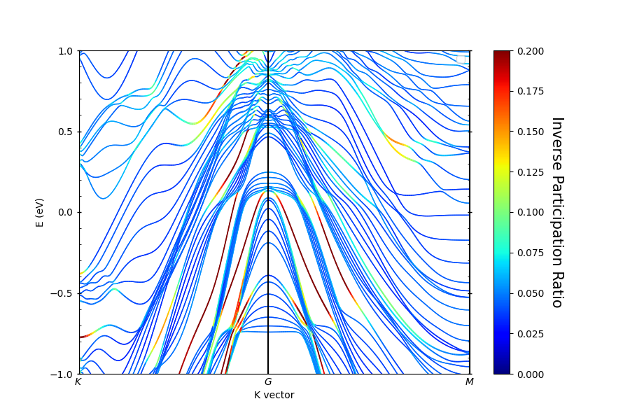
Topologically-protected surface states in \(Bi_2Se_3\)

The first example is the detection of topologically-protected surface states in \(Bi_2Se_3\), [zhang2009]. The whole slab has six van der Waals layers (quintuple layers), each is five atom thick. The surface states localize on the outer quintuple layers, in contrast a extended state cover the six quintuple layers. The ratio between the localization of both types of states is 1 to 3, and the $IPR$ has enough resolution to provide a clear visual identification. The PyProcar code is:

pyprocar.bandsplot(dirname=bi2se3_data_dir,
                   elimit=[-1.0,1.0],
                   mode='ipr',
                   code='vasp',
                   spins=[0],
                   clim=[0,0.2])

            ----------------------------------------------------------------------------------------------------------
            There are additional plot options that are defined in the configuration file.
            You can change these configurations by passing the keyword argument to the function.
            To print a list of all plot options set `print_plot_opts=True`

            Here is a list modes : plain , parametric , scatter , atomic , overlay , overlay_species , overlay_orbitals , ipr
            ----------------------------------------------------------------------------------------------------------


            WARNING : `fermi` is not set! Set `fermi={value}`. The plot did not shift the bands by the Fermi energy.
            ----------------------------------------------------------------------------------------------------------


(<Figure size 900x600 with 2 Axes>, <Axes: xlabel='K vector', ylabel='E (eV)'>)

\(NV^-\) defect in diamond

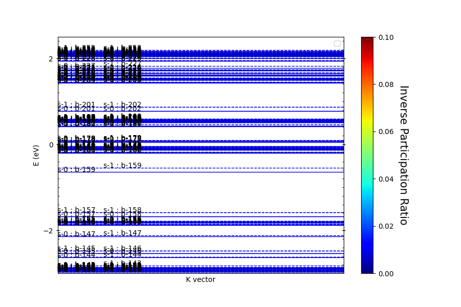
The second example is the \(NV^-\) defect in diamond, it is a negatively charged N substitution plus an adjacent vacancy. This defect if of interest as a source of single photons. Its ground state is a triplet, allowing the control of the spin by microwave radiation.[DOHERTY2013] The supercell has 215 atoms, hence \(IPR\to0\) for bulk states (blue lines). Several defect levels lie within the fundamental band gap of diamond (dark red lines). The closest levels to the Fermi energy are double degenerate (i.e. triplet), but only occupied for the spin majority. Hence, according to the optical transition takes place between the bands with index \(430\to431\) or \(430\to432\) of the spin channel labelled spin-1. The calculation of the main emission line involves a calculation of the excited state, which can be simulated by fixing the occupations of the mentioned levels, i.e. the \(\Delta\) SCFmethod.[Jin2021] The pyprocar code is:

pyprocar.bandsplot(dirname=C_data_dir,
                   elimit=[-3.0,2.5],
                   mode='ipr',
                   code='vasp',
                   spins=[0,1],
                   clim=[0,0.1])

            ----------------------------------------------------------------------------------------------------------
            There are additional plot options that are defined in the configuration file.
            You can change these configurations by passing the keyword argument to the function.
            To print a list of all plot options set `print_plot_opts=True`

            Here is a list modes : plain , parametric , scatter , atomic , overlay , overlay_species , overlay_orbitals , ipr
            ----------------------------------------------------------------------------------------------------------


            WARNING : `fermi` is not set! Set `fermi={value}`. The plot did not shift the bands by the Fermi energy.
            ----------------------------------------------------------------------------------------------------------

z:\research projects\pyprocar\pyprocar\plotter\ebs_plot.py:607: UserWarning: Attempting to set identical low and high xlims makes transformation singular; automatically expanding.
  self.ax.set_xlim(interval)
Atomic plot: bands.shape  : (2, 540, 2)
Atomic plot: spd.shape    : (2, 540, 215, 1, 9, 2)
Atomic plot: kpoints.shape: (2, 3)

(<Figure size 900x600 with 2 Axes>, <Axes: xlabel='K vector', ylabel='E (eV)'>)