Example of finding the bandgap

The ElectronicBandStructure is used to handle the information related to the electronic band structure.

General Format

import pyprocar
pyprocar.io.Parser(code="vasp", dir=data_dir)

Downloading example

 data_dir = pyprocar.download_example(save_dir='',
                             material='Fe',
                             code='vasp',
                             spin_calc_type='non-spin-polarized',
                             calc_type='bands')

# sphinx_gallery_thumbnail_number = 1

import pyvista as pv

# You do not need this. This is to ensure an image is rendered off screen when generating exmaple gallery.
pv.OFF_SCREEN = True

importing pyprocar and specify the local data_dir

import os

import numpy as np

import pyprocar

data_dir = os.path.join(
    pyprocar.utils.DATA_DIR, "examples", "Fe", "vasp", "non-spin-polarized", "fermi"
)

Initialize the parser object and get the ElectronicBandStructure

parser = pyprocar.io.Parser(code="vasp", dir=data_dir)
ebs = parser.ebs
e_fermi = parser.ebs.efermi
structure = parser.structure
# Apply symmetry to get a full kmesh
if structure.rotations is not None:
    ebs.ibz2fbz(structure.rotations)

You can print the object to see some information about the Band Structure

print(ebs)

Enectronic Band Structure
------------------------
Total number of kpoints  = 3375
Total number of bands    = 8
Total number of atoms    = 1
Total number of orbitals = 9

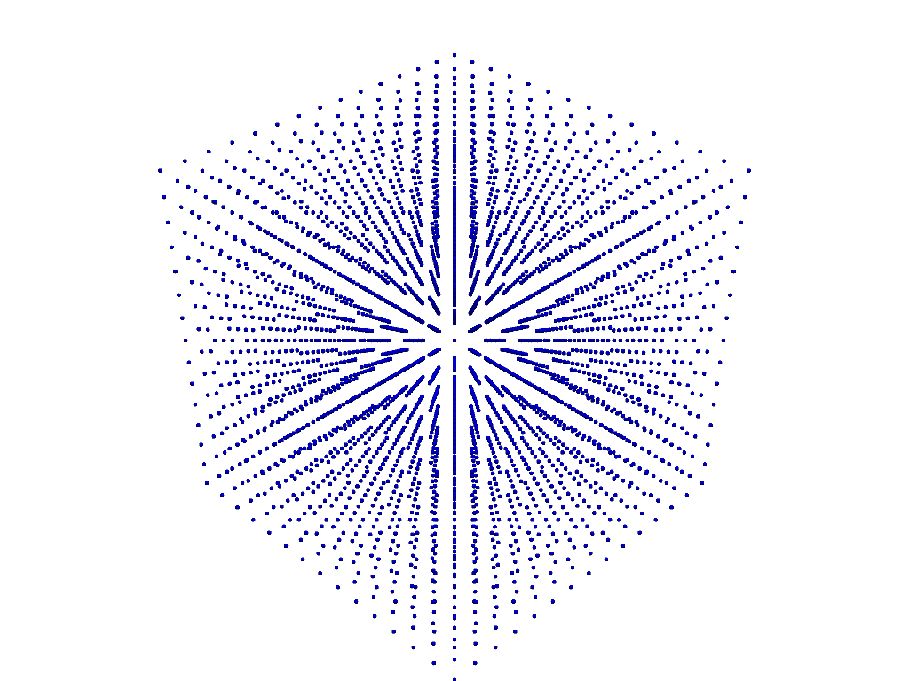
Let’s plot the kpoints

p = pv.Plotter()
p.add_mesh(ebs.kpoints, color="blue", render_points_as_spheres=True)
p.show()

Other properties

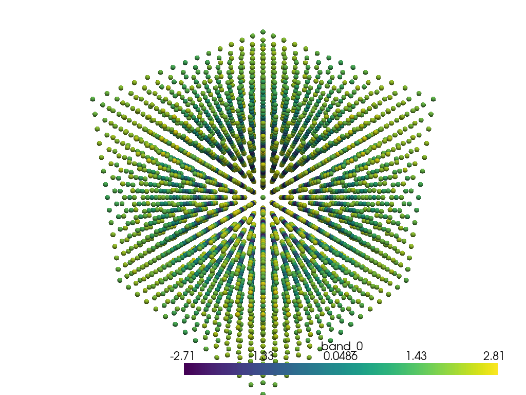
Bands

kpoints = pv.PolyData(ebs.kpoints)
kpoints["band_0"] = ebs.bands[:, 0, 0]

p = pv.Plotter()
p.add_mesh(
    kpoints,
    color="blue",
    scalars="band_0",
    render_points_as_spheres=True,
    point_size=10,
)
p.show()

Projections

print(f"Electron projected shape: {ebs.projected.shape}")
kpoints["band_0-atom_0-orbital_5-spin-0"] = ebs.projected[:, 0, 0, 0, 4, 0]

p = pv.Plotter()
p.add_mesh(
    kpoints,
    color="blue",
    scalars="band_0-atom_0-orbital_5-spin-0",
    render_points_as_spheres=True,
    point_size=10,
)
p.show()

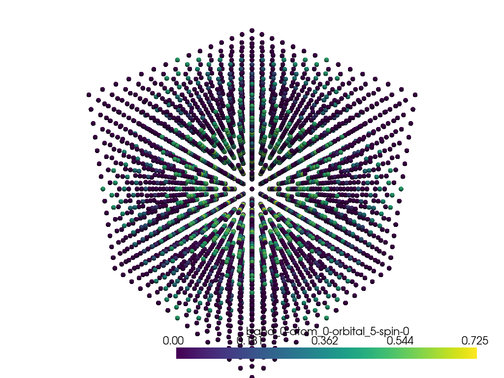
Electron projected shape: (3375, 8, 1, 1, 9, 1)

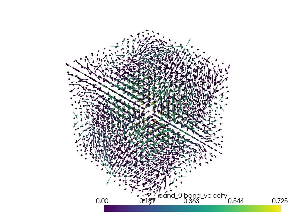
Gradients

print(f"Band gradient shape: {ebs.bands_gradient.shape}")
kpoints["band_0-gradients"] = ebs.bands_gradient[:, 0, 0, :]

# Use the Glyph filter to generate arrows for the vectors
arrows = kpoints.glyph(orient="band_0-gradients", scale=False, factor=0.08)
p = pv.Plotter()
p.add_mesh(arrows, scalar_bar_args={"title": "band_0-band_velocity"})
p.show()

ij,uvwabj->uvwabi
Band gradient shape: (3375, 8, 1, 3)

Band/Fermi velocities

print(f"Fermi velocity shape: {ebs.fermi_velocity.shape}")
print(f"Fermi speed shape: {ebs.fermi_speed.shape}")
kpoints["band_0-band_velocity"] = ebs.fermi_velocity[:, 0, 0, :]
kpoints["band_0-band_speed"] = ebs.fermi_speed[:, 0, 0]

arrows = kpoints.glyph(orient="band_0-band_velocity", scale=False, factor=0.08)
p = pv.Plotter()
p.add_mesh(
    kpoints,
    scalars="band_0-band_speed",
    render_points_as_spheres=True,
    point_size=0.1,
    show_scalar_bar=False,
)
p.add_mesh(arrows, scalar_bar_args={"title": "band_0-band_velocity"})
p.show()

Fermi velocity shape: (3375, 8, 1, 3)
Fermi speed shape: (3375, 8, 1)

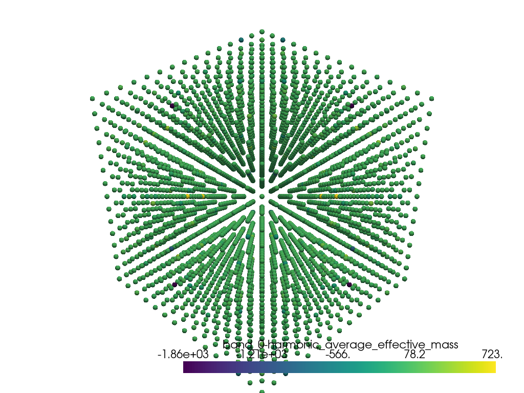
Effective mass

print(
    f"Harmonic average effective mass shape: {ebs.harmonic_average_effective_mass.shape}"
)
kpoints["band_0-harmonic_average_effective_mass"] = ebs.harmonic_average_effective_mass[
    :, 0, 0
]

p = pv.Plotter()
p.add_mesh(
    kpoints,
    scalars="band_0-harmonic_average_effective_mass",
    render_points_as_spheres=True,
    point_size=10,
)
p.show()

ij,uvwabcj->uvwabci
Harmonic average effective mass shape: (3375, 8, 1)