Plotting with Configurations in pyprocar

This example illustrates how to utilize various configurations for plotting the 3D Fermi surface using the pyprocar package. It provides a structured way to explore and demonstrate different configurations for the plot_fermi_surface function.

Symmetry does not currently work! Make sure for Fermi surface calculations to turn off symmetry.

Preparation

Before diving into plotting, we need to download the example files. Use the following code to do this. Once downloaded, specify the data_dir to point to the location of the downloaded data.

Downloading example

 data_dir = pyprocar.download_example(save_dir='',
                             material='Fe',
                             code='vasp',
                             spin_calc_type='non-spin-polarized',
                             calc_type='fermi')

import pyvista
# You do not need this. This is to ensure an image is rendered off screen when generating example gallery.
pyvista.OFF_SCREEN = True

import os
import pyprocar

data_dir = f"{pyprocar.utils.ROOT}{os.sep}data{os.sep}examples{os.sep}Fe{os.sep}vasp{os.sep}non-spin-polarized{os.sep}fermi"

# First create the FermiHandler object, this loads the data into memory. Then you can call class methods to plot.
# Symmetry only works for specific space groups currently.
# For the actual calculations turn off symmetry and set 'apply_symmetry'=False.
fermiHandler = pyprocar.FermiHandler(
                                    code="vasp",
                                    dirname=data_dir,
                                    apply_symmetry=True)

WARNING : Fermi Energy not set! Set `fermi={value}`. By default, using fermi energy found in given directory.
---------------------------------------------------------------------------------------------------------------

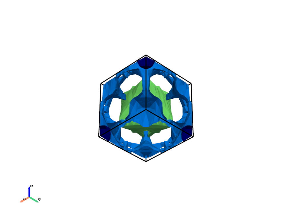
# Section 1: Plain Mode
# ++++++++++++++++++++++++++++++++++++++++++++++++++++++++++++++++++++++++++++++
#
# This section demonstrates how to plot the 3D Fermi surface using default settings.


# Section 1: Locating and Printing Configuration Files
# ++++++++++++++++++++++++++++++++++++++++++++++++++++++++++++++++++++++++++++++
#
# This section demonstrates where the configuration files are located in the package.
# It also shows how to print the configurations by setting print_plot_opts=True.
#

# Path to the configuration files in the package
config_path = os.path.join(pyprocar.__path__[0], 'cfg')
print(f"Configuration files are located at: {config_path}")

fermiHandler.plot_fermi_surface(mode="plain",
                                show=True,
                                print_plot_opts=True)

Configuration files are located at: z:\research projects\pyprocar\pyprocar\cfg

                --------------------------------------------------------
                There are additional plot options that are defined in a configuration file.
                You can change these configurations by passing the keyword argument to the function
                To print a list of plot options set print_plot_opts=True

                Here is a list modes : plain , parametric , spin_texture , overlay
                Here is a list of properties: fermi_speed , fermi_velocity , harmonic_effective_mass
                --------------------------------------------------------

surface_cmap : {'value': 'jet', 'description': 'Controls the colormap of the surface'}
surface_color : {'value': None, 'description': 'Controls the color of the surface'}
spin_colors : {'description': 'The colors for the plot lines.', 'value': [None, None]}
surface_bands_colors : {'value': [], 'description': 'Controls the color of the surface per band'}
surface_opacity : {'value': 1.0, 'description': 'Controls the opacity of the surface'}
surface_clim : {'value': None, 'description': 'Controls the color scale on the surface'}
extended_zone_directions : {'value': None, 'description': 'Controls how many zone to generate. This is a list of directions to generates. Ex: [[1,0,0],[0,0,1]]'}
supercell : {'value': [1, 1, 1], 'description': 'Controls how many the supercell size used to generate the fermi surface'}
projection_accuracy : {'value': 'high', 'description': 'Controls the projection algorithmuse. Either high or normal'}
interpolation_factor : {'value': 1, 'description': 'Controls the interpolation factor used on the fermi surface'}
brillouin_zone_style : {'value': 'wireframe', 'description': 'Controls the wireframe style of the brillouin zone'}
brillouin_zone_line_width : {'value': 3.5, 'description': 'Controls the linewidth of the brillouin zone'}
brillouin_zone_color : {'value': 'black', 'description': 'Controls the color of the wireframe of the brillouin zone'}
brillouin_zone_opacity : {'value': 1.0, 'description': 'Controls the opacity of the wireframe of the brillouin zone'}
texture_cmap : {'value': 'jet', 'description': 'Controls the colormap of the texture'}
texture_color : {'value': None, 'description': 'Controls the color of the texture'}
texture_size : {'value': 0.1, 'description': 'Controls the size of the texture'}
texture_scale : {'value': False, 'description': 'Controls the scaling of the texture'}
texture_opacity : {'value': 1.0, 'description': 'Controls the opacity of the texture'}
add_axes : {'value': True, 'description': 'Controls if there should be direction axes'}
x_axes_label : {'value': 'Kx', 'description': 'Controls kx axis label'}
y_axes_label : {'value': 'Ky', 'description': 'Controls ky axis label'}
z_axes_label : {'value': 'Kz', 'description': 'Controls kz axis label'}
axes_label_color : {'value': 'black', 'description': 'Controls axes label color'}
axes_line_width : {'value': 6, 'description': 'Controls the linewdith of th axes label'}
add_scalar_bar : {'value': True, 'description': 'Controls if there is a colorbar'}
scalar_bar_labels : {'value': 6, 'description': 'Controls the scalar bar labels'}
scalar_bar_italic : {'value': False, 'description': 'Controls the label italic style'}
scalar_bar_bold : {'value': False, 'description': 'Controls the label bold style'}
scalar_bar_title : {'value': None, 'description': 'Controls scalar bar title font size'}
scalar_bar_title_font_size : {'value': None, 'description': 'Controls scalar bar title font size'}
scalar_bar_label_font_size : {'value': None, 'description': 'Controls scalar bar label font size'}
scalar_bar_position_x : {'value': 0.4, 'description': 'Controls scalar bar x position'}
scalar_bar_position_y : {'value': 0.01, 'description': 'Controls scalar bar y position'}
scalar_bar_color : {'value': 'black', 'description': 'Controls scalar bar outline color'}
background_color : {'value': 'white', 'description': 'Controls the background color'}
orbit_gif_n_points : {'value': 36, 'description': 'Controls the number of point on the orbit'}
orbit_gif_step : {'value': 0.05, 'description': 'Controls the step size of the orbit'}
orbit_mp4_n_points : {'value': 36, 'description': 'Controls the number of point on the orbit'}
orbit_mp4_step : {'value': 0.05, 'description': 'Controls the step size of the orbit'}
plotter_offscreen : {'value': False, 'description': 'Controls whether the plotter renders offscreen'}
plotter_camera_pos : {'value': [1, 1, 1], 'description': 'Controls the caemera position of the plotter'}
isoslider_title : {'value': 'Energy iso-value', 'description': 'Controls title of the isoslider'}
isoslider_style : {'value': 'modern', 'description': 'Controls isoslider  style'}
isoslider_color : {'value': 'black', 'description': 'Controls isoslider color'}
cross_section_slice_linewidth : {'value': 5.0, 'description': 'Controls the linewidth of the slice\\'}
cross_section_slice_show_area : {'value': False, 'description': 'Controls wheather to show the cross section area'}
arrow_size : {'description': 'The arrow size for the spin texture', 'value': 3}
Bands Near Fermi :  [2, 3, 4, 5]

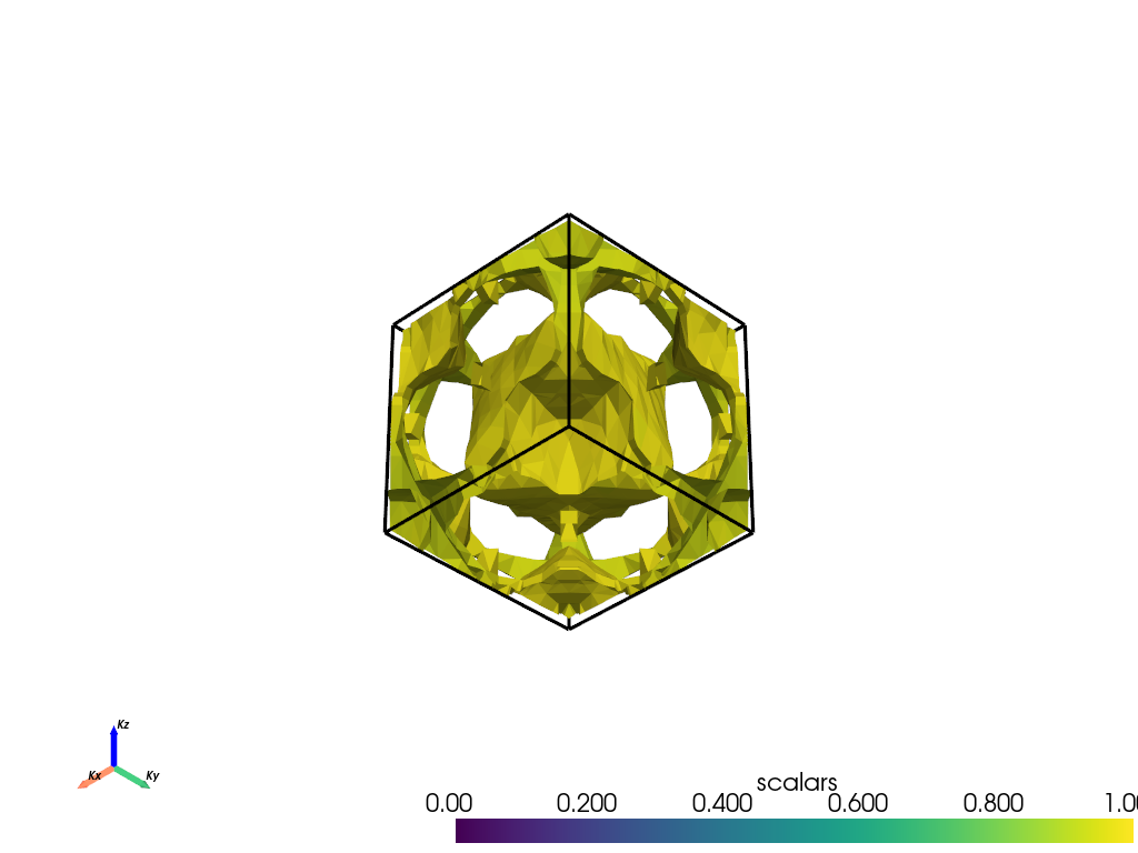
# Section 2: Parametric Mode with Custom Settings
# ++++++++++++++++++++++++++++++++++++++++++++++++++++++++++++++++++++++++++++++
#
# This section demonstrates how to customize the appearance of the 3D Fermi surface in parametric mode.
# We'll adjust the colormap, color limits, and other settings.

atoms=[0]
orbitals=[4,5,6,7,8]
spins=[0]
fermiHandler.plot_fermi_surface(mode="parametric",
                              atoms=atoms,
                              orbitals=orbitals,
                              spins=spins,
                              surface_cmap='viridis',
                              surface_clim=[0, 1],
                              show=True)

                --------------------------------------------------------
                There are additional plot options that are defined in a configuration file.
                You can change these configurations by passing the keyword argument to the function
                To print a list of plot options set print_plot_opts=True

                Here is a list modes : plain , parametric , spin_texture , overlay
                Here is a list of properties: fermi_speed , fermi_velocity , harmonic_effective_mass
                --------------------------------------------------------

Bands Near Fermi :  [2, 3, 4, 5]