Showing how to get van alphen fequencies from the fermi surface

Symmetry does not currently work! Make sure for fermi surface calculations turn off symmetry

Van alphen fequencies example. De has van alphen frequencies (F) in terms of extremal fermi surface areas (A) is given below. To compare the theoretical freuqencies we will compare with the results taken from the experimental paper “The Fermi surfaces of copper, silver and gold. I. The de Haas-Van alphen effect”(https://doi.org/10.1098/rsta.1962.0011).

\[ \begin{align}\begin{aligned}F = \frac{ c \hbar A }{ 2 \pi e } !(cgs)\\e = 4.768e^{-10} !statcoulombs\\c = 3.0e^{10} !cm/s\\\hbar = 1.0546e^{-27} !erg*s\end{aligned}\end{align} \]

First download the example files with the code below. Then replace data_dir below.

Downloading example

 data_dir = pyprocar.download_example(save_dir='',
                             material='Au',
                             code='vasp',
                             spin_calc_type='non-spin-polarized',
                             calc_type='fermi')

# sphinx_gallery_thumbnail_number = 1

import pyvista
# You do not need this. This is to ensure an image is rendered off screen when generating exmaple gallery.
pyvista.OFF_SCREEN = True

importing pyprocar and specifying local data_dir

import os
import pyprocar

data_dir = f"{pyprocar.utils.ROOT}{os.sep}data{os.sep}examples{os.sep}Au{os.sep}vasp{os.sep}non-spin-polarized{os.sep}fermi"


# First create the FermiHandler object, this loads the data into memory. Then you can call class methods to plot
# Symmetry only works for specfic space groups currently.
# For the actual calculations turn off symmetry and set 'apply_symmetry'=False
fermiHandler = pyprocar.FermiHandler(
                                    code="vasp",
                                    dirname=data_dir,
                                    apply_symmetry=True)

WARNING : Fermi Energy not set! Set `fermi={value}`. By default, using fermi energy found in given directory.
---------------------------------------------------------------------------------------------------------------

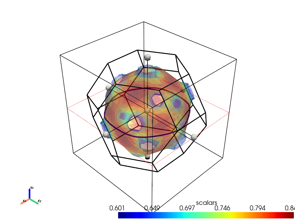
Maximal cross sectional area along the (0,0,1)

fermiHandler.plot_fermi_cross_section_box_widget(
                            bands=[5],
                            slice_normal=(0,0,1),
                            slice_origin=(0,0,0),
                            surface_opacity=0.40,
                            mode="parametric",
                            show=True)

                --------------------------------------------------------
                There are additional plot options that are defined in a configuration file.
                You can change these configurations by passing the keyword argument to the function
                To print a list of plot options set print_plot_opts=True

                Here is a list modes : plain , parametric , spin_texture , overlay
                Here is a list of properties: fermi_speed , fermi_velocity , harmonic_effective_mass
                --------------------------------------------------------

Bands Near Fermi :  [5]
Bands being used if bands=None:  [0]

In the above figure we can see the cross section area is \(A = 4.1586 Ang^{-2} = 4.1586e^{16} cm^{-2} (cgs)\).

\(F = \frac{ c \hbar A }{ 2 \pi e } = 4.365e^8 G\)

\(F_{exp} = 4.50e^7 G\)

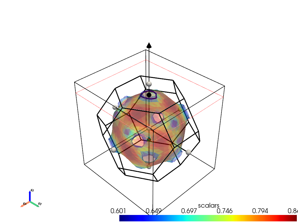
Minimal cross sectional area along the (0,0,1)

fermiHandler.plot_fermi_cross_section_box_widget(
                                bands=[5],
                                slice_normal=(0,0,1),
                                slice_origin=(0,0,1.25),
                                surface_opacity=0.40,
                                mode="parametric",
                                show=True,)

                --------------------------------------------------------
                There are additional plot options that are defined in a configuration file.
                You can change these configurations by passing the keyword argument to the function
                To print a list of plot options set print_plot_opts=True

                Here is a list modes : plain , parametric , spin_texture , overlay
                Here is a list of properties: fermi_speed , fermi_velocity , harmonic_effective_mass
                --------------------------------------------------------

Bands Near Fermi :  [5]
Bands being used if bands=None:  [0]

In the above figure we can see the cross section area is \(A = 0.1596 Ang^{-2} = 0.1596e^{16} cm^{-2} (cgs)\).

\(F = \frac{ c \hbar A }{ 2 \pi e } = 1.68e^7 G\)

\(F_{exp} = 1.50e^7 G\)

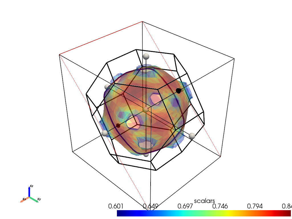
Extremal cross sectional area along the (0,1,1)

fermiHandler.plot_fermi_cross_section_box_widget(
                                bands=[5],
                                slice_normal=(0,1,1),
                                slice_origin=(0,0,0),
                                surface_opacity=0.40,
                                mode="parametric",
                                show=True,)

                --------------------------------------------------------
                There are additional plot options that are defined in a configuration file.
                You can change these configurations by passing the keyword argument to the function
                To print a list of plot options set print_plot_opts=True

                Here is a list modes : plain , parametric , spin_texture , overlay
                Here is a list of properties: fermi_speed , fermi_velocity , harmonic_effective_mass
                --------------------------------------------------------

Bands Near Fermi :  [5]
Bands being used if bands=None:  [0]

In the above figure we can see the cross section area is \(A = 4.3956 Ang^{-2} = 4.3956e^{16} cm^{-2} (cgs)\).

\(F = \frac{ c \hbar A }{ 2 \pi e } = 4.61e^8 G\)

\(F_{exp} = 4.85e^8 G\)